Earthing System Analysis for Steel Tower Carrying 33kV Line

Adebayo Adeniyi David; Ifeagwu Emmanuel Ncheta; Ogunsakin Olatunji Rufus

doi:doi:10.11648/j.es.20240902.11

Research Article |

| Peer-Reviewed

Earthing System Analysis for Steel Tower Carrying 33kV Line

Adebayo Adeniyi David^*

, Ifeagwu Emmanuel Ncheta, Ogunsakin Olatunji Rufus

Published in Engineering Science (Volume 9, Issue 2)

Received: 14 February 2024 Accepted: 8 March 2024 Published: 29 June 2024

Views: Downloads:

Download PDF

Share This Article

Twitter
Linked In
Facebook

Abstract

This study examines the critical analysis of earthing systems connected to steel towers that carry 33 kV power lines. Ensuring the safety and dependability of power transmission infrastructure becomes crucial in light of the growing demand for energy. By utilizing sophisticated computational methodologies and simulation approaches, this research carefully investigates how well the earthing system performs in various operational circumstances and fault scenarios. A thorough modeling technique is used in the analysis, which considers a number of variables including fault currents, tower design, soil resistivity, and grounding electrode configurations. In order to give a comprehensive understanding of the behavior of the system and its consequences for operational reliability, the study simulates many situations, including normal operation and fault occurrences. By using sophisticated numerical simulations and sensitivity analysis, the research pinpoints important factors affecting the earthing system's efficiency and suggests creative optimization techniques. These optimization techniques could involve changing the location of the grounding electrode, improving the materials used in the conductor, or putting additional safety precautions in place. The researcher's conclusions have important ramifications for the engineering community since they provide practical advice on how to strengthen the security and robustness of power transmission networks. The study adds to the continuous efforts to improve the efficiency and dependability of electrical grids by addressing potential weaknesses in the architecture of the earthing system. This thorough study advances the field of earthing system engineering by offering a solid platform for next studies and real-world implementations. Through this work, we can better understand the dynamics of earthing systems and optimization methodologies, which will help build more resilient and sustainable power transmission infrastructure that can adapt to society's changing energy needs.

Published in	Engineering Science (Volume 9, Issue 2)
DOI	10.11648/j.es.20240902.11
Page(s)	21-38
Creative Commons	This is an Open Access article, distributed under the terms of the Creative Commons Attribution 4.0 International License (http://creativecommons.org/licenses/by/4.0/), which permits unrestricted use, distribution and reproduction in any medium or format, provided the original work is properly cited.
Copyright	Copyright © The Author(s), 2024. Published by Science Publishing Group

Keywords

Earthing, Grounding, Towers, Electrodes, Analysis, Grid

1. Introduction

Safety is paramount in the Nigerian energy supply sector, yet it is a concern that is often overlooked. Concerns about the safety of energy users have been raised by various stakeholders including the government, employers, labor organizations, and the general public, as well as power supply authorities

[1]

. Improper handling of electricity poses significant risks, potentially leading to irreversible harm to individuals and property. Therefore, ensuring the effectiveness and responsiveness of safety devices and protection mechanisms is crucial.

The efficiency of the earthing system plays a pivotal role in ensuring safety and reliability in electrical installations. It directly affects the coordination of relays and the performance of circuit breakers in substations

[2]

. Weaknesses in the earthing system of substations are a major contributor to electrical risks faced by maintenance workers and end-users alike. To mitigate these risks and prevent electrical hazards, it is imperative to evaluate and enhance the earthing systems of distribution substations

[3]

Furthermore, the electrical characteristics of various conductors and transformers are fundamental considerations in designing and optimizing earthing systems. For instance, the resistance per kilometer length of bare Aluminum multi-stranded conductors (AAC-type) and Steel Reinforced (ACSR-type) conductors are key parameters to assess

[4]

. Additionally, the specifications of transformers, such as the 333/11 kV and 132/33 kV transformers, are crucial in determining the overall performance of the electrical system

[5]

To facilitate accurate analysis and evaluation of earthing systems, sophisticated tools like the Electrical Transient Analyzer Program (ETAP) are utilized for simulation and assessment purposes

[6]

. These tools enable engineers to model and simulate various scenarios, allowing for comprehensive analysis and optimization of earthing systems.

2. Materials and Method

Materials and Systems Used.

The following materials were considered for this study.

1) The Distributed Generation technology used is gas turbine synchronous generator. The rated power is 3 MW, generating at 11 kV and frequency is 50 Hz.

2) 150 sq mm cross sectional area of Aluminum overhead conductor.

3) Pre-calculated resistance per km length of bare Aluminum multi-stranded conductor (AAC-type for 150 mn2 is 0.1825 ohms/km. Pre-calculated resistance per km length of bare Aluminum multi-stranded conductor Steel Reinforced (ACSR-type) for 150 mm² is 0.l828 ohms/km.

4) 33/11 kV and 132/33 kV transformers.

5) Electrical Transient Analyzer Program (ETAP) software used for simulation.

2.1. System Specifications

DG power rating = 3MW- 20 MW Voltage level of Feeder = 33 kV

Frequency 50Hz

Conductor size: 150 mm2 (AAC)

Type of transformer: 33/11 kV and 132/33 kV

2.2. Network Configuration

There are five Transmission load centers in Port Harcourt Region. These are:

1) Port Harcourt Mains, also known as Z2,

2) Port Harcourt Town, popularly called Z4 at D-Line Quarter of Port Harcourt Town,

3) Afam,

4) Elenlewon and

5) Rumuosi Transmission Stations.

Table 1. 132/33k V Port Harcourt TCN Transmitting Stations.

	Transmission Station	Transformer Rating	Number of 33 kV Feeders	Name of Feeder
1	Afam Station	45 MVA, 132/33 kV	2	Ndokil (Afam Town) Komkom
2	Elelenwo	2x60 MVA, 132/33 kV	6	Old Oyigbo Igbo Etche Timber RSTV Onne/Elenwo Bori
3	PH Mains Z2, Oginigba.	3x 60 MVA, 132/33 kV	10	Trans-Amadi Rainbow Oyigbo Refinery Rumuduomaya Abuloma Woji Rumuola Akanni Airport Spare
4	Rumuosi	2x40 MVA 132/33 Kv	4	New Airport Rukpokwu NTA UPTH
5	PH Town Z4	2x30 MVA 132/33 kV 1x45MVA 132/33 kV 1x6O MVA 132/33 kV	9	Secretariat Borokiri Silverbird UTC Rumuolumini Amadi Junction Amadi Junction Amadi Junction UST

One 330 kV line from Enugu transmission station and one 132kV line from Alaoji transmission station supply electric power to Afam Transmission station as shown in Figure 2. Afam transmission station supplies power at 132 kV level to all the transmission substations in Port Harcourt metropolis apart from Rumuosi transmission substation. Two 132 kV lines go to Elelenwo transmission substation, two 132 kV lines go to Port Harcourt Mains transmission station. From the two 132 kV lines that supply power to Port Harcourt mains, two lines are tapped to Port Harcourt Town Z4, Amadi Junction transmission station. One 132 kV line connects Port Harcourt Mains to Rumuosi transmission station. One 132 kV line connects Trans Amadi Gas turbine generation station to Port Harcourt Mains transmission station. There are two 132 kV parallel lines that supply electric power to Rumuosi transmission station from Omoku Gas Turbine. The gas turbine generating station consists of 6 x 25 MW Gas Turbine Generators, 6 x 25/35 MVA, 11/33 kV transformers and 2 x. 60/75 MVA, 33/132 kV transformers. There is one outgoing 132kV circuit that connects this generating station with Port Harcourt Mains Transmission station. The parameters of these transmission stations are shown in Table 1.

2.3. Design Equations

The following are the design equations for the Earthing System Analysis for Steel Tower Carrying 33kV line

[7]

2.3.1. Determination of the Earth Grid Resistance

R = P [\frac{1}{lr} + \frac{1}{\sqrt{20 A}} (1 + \frac{1}{1 + \sqrt[H]{\frac{20}{A}}})]

(1)

Where;

ℓ= Soil resistivity (52/m)

A= The occupied ground grid area (m2)

𝐿𝑇= The total conductors length buried (m)

h= the grid depth (m)

The sub transmission station earthing comprises six (6) Pits, each pit has their evaluated value as shown in Table 2 to Table 9. Initial Parameters Data Collected from the Sub Transmission Station Site Current probe dc in all the tests carried out is placed at 20m, Table 2 to Table 9 below shows the earth resistance values of each pit from pit 1 to pit 8.

Table 2. The Distance and the Earth Resistance Values of Pit 1.

S/No	Distance (M)	Resistance
1	4	1.17
2	8	1.24
3	12	1.39

Actual earth resistance for pit 1=1.17

Table 3. The Distance and the Earth Resistance Values of Pit 2.

S/No	Distance (M)	Resistance
1	4	1.21
2	8	0.57
3	12	0.64

Actual earth resistance for pit 2=0.57

Table 4. The Distance and the Earth Resistance for Pit 3.

S/No	Distance (M)	Resistance
1	4	1.25
2	8	1.29
3	12	1.41

Actual earth resistance for pit 3=1.25

Table 5. The Distance and the Earth Resistance for Pit 4.

S/No	Distance (M)	Resistance
1	4	4.25
2	8	3.26
3	12	2.42

Actual earth resistance for pit 4=3.25

Table 6. The Distance and the Earth Resistance for Pit 5.

S/No	Distance (M)	Resistance
1	4	0.25
2	8	0.41
3	12	0.55

Actual earth resistance for pit 5=0.45

Table 7. The Distance and the Earth Resistance for Pit 6.

S/No	Distance (M)	Resistance
1	4	0.66
2	8	1.01
3	12	0.83

Actual earth resistance for pit 6=0.57

Table 8. The Distance and the Earth Resistance for Pit 7.

S/No	Distance (M)	Resistance
1	4	2.10
2	8	1.40
3	12	2.11

Actual earth resistance for pit 7=1.87

Table 9. The Distance and the Earth Resistance for Pit 8.

S/No	Distance (M)	Resistance
1	4	3.01
2	8	2.45
3	12	1.47

Actual earth resistance for pit 8=2.25

Introductory Design of 132kV OHL substation establishing contextual analysis boundaries are given Slope Coefficient,

U = 0.55

Potential Probe Distance, DPT = 10.97M

Actual Resistance,

R = 0.59Ω 60 MVA

Transformer = 132/33KV

Lightning Arresters = 0.20Ω

Line Gantry = 0.20Ω 300KVA 33/0.415KV

Earthing Transformer Body = 0.43Ω

Table 10. Continuity Checks of Equipment to Earthing Grid System.

S/No	Equipment	STATUS
1	All Panels in Switchgear Room	Continuous
2	All panels in battery	Continuous
3	All panels in communication room	Continuous
4	132kv lightning arresters	Continuous
5	Perimeter lighting	Continuous
6	Perimeter fencing	Continuous
7	Control room	Continuous
8	All gantry support	Continuous

Resistivity of Soil and Surface Layer

The soil edifice can be calculated based on its soil resistivity, (stream bank development may be 1.5 ohm-meters resistivity esteem, though dry sand or stone may have norms of 10,000 ohm-meters), as shown in Table 11.

Table 11. The Depth of Earth Conductor.

No.	Soil	Resistivity	Economical depth
	in ohms/meter		Buried in meters
1	50 –100		0.5
2	100	–400	1.0
3	400	–1000	1.5

Earth Resistance Determination of the Sub Transmission Station Site

Soil resistivity (ℓ) = 100Ω/m

Crush rock resistivity (ℓ) = 2566Ω/m

Earth Resistance Determination of the Sub Transmission Station Site

Soil resistivity (ℓ) = 100Ω/m

Crush rock resistivity (ℓ) = 2566Ω/m

Length of grid (𝐿) = 200ft=70m

Breath of grid (𝐵) = 200ft = 70m)

Parallel conductors = 11 × 11 = 121

Depth of earth grid (ℎ) = 6ft = 1.8288m

Number of electrodes (𝑁) = 22

Length of electrodes (𝑁) = 6𝑓𝑡 = 1.8288𝑚

2.3.2. Determination of Thickness of Crushed Rock

(ℎ𝑠) = 0.5𝑓𝑡= 0.1524 (2)

2.3.3. Determination of Area Occupied by the Ground Grid

A = L \times B

(3)

Total buried length of conductors

[8]

L_{T} = (11 \times L) + (11 \times B) + (N_{r} \times N_{I})

(3)

Surface layer derating factor

[9]

C_{S} = 1 - \frac{0.09 (1 - \frac{t}{t_{s}})}{2 h_{s} + 0.09}

(4)

Where, ℓ = Soil resistivity ℓ𝑠= Crush rock resistivity and Tolerable Touch and Step Potential For 70Kg Person

E_{touch 70} = (100 + 1.5 \times C_{s} \times l_{s}) \times \frac{0.157}{\sqrt{ts}}

(5)

Where; 𝐸𝑡𝑜𝑢𝑐ℎ70= touch Potential limit 𝐶𝑠= surface layer derating factor ℓ𝑠= resistivity of crush rock 𝑡𝑠= exposure time or shock duration =0.5sec

E_{step 70} = (1000 + 6 \times c_{S} \times L_{S}) \times \frac{0.157}{\sqrt{ts}}

(6)

Where 𝐸𝑠𝑡𝑒𝑝= The Step Potential

2.3.4. Determination of Decremental Factor (𝐷𝑓)

D_{t} = \sqrt{1 + \frac{T_{a}}{t_{f}} (1 - e^{\frac{- 2 tf}{Ta}})}

(7)

Hence; Ta= dc time offset in seconds (is a constant)

tf = duration of fault time

Note that

[10]

;

T_{a} = (\frac{X}{R}

)(

\frac{1}{2 πf})

(8)

Hence

\frac{X}{R} = fault location ratio at 15

f= frequency=50hz

Grid Current Maximum (IG),

[11]

I_{G} = S_{f} \times D_{f} \times C_{P} \times I_{g}

(9)

Where; Sf = fault current division factor

Df = Decremental factor

Cp = 𝐶𝑜𝑟𝑟𝑒𝑐𝑡𝑖𝑣𝑒 𝑝𝑟𝑜𝑗𝑒𝑐𝑡𝑖𝑜𝑛 𝑓𝑎𝑐𝑡𝑜𝑟

Ig= Symmetrical short circuit current

2.3.5. Determination of Ground Potential Rise (GRR)

GPR = R_{g} \times I_{G}

(10)

2.3.6. Determination of Geometric Factor

n = n_{a} \times n_{b} \times n_{c \times} n_{d}

(11)

q_{a} = \frac{2 LC}{L_{p}} = \frac{2 \times (11 \times l) + (11 \times B)}{2 (L + B)}

(12)

Where

q_{b}

=l, for square grids

q_{c} =

for square and rectangular

q_{d} = 1

for square and rectangular and L shaped.

2.3.7. Determination of Spacing Between Parallel Grid Conductor

\frac{1}{2}

(

\frac{B}{nr - 1} + \frac{l}{nc - 1}

) (13)

Where B=width of grid

L=length of grid

Nr=number of parallel rods

NC=number pf parallel conducts

2.3.8. Determination of Weighting Factor

The corner mesh earth electrodes for weighing factor

[12]

K_{h} = \sqrt{1 + h}

(14)

Where

K_{h}

=weighting factor for depth of buried rod

{(K}_{m})

2.3.9. Determination of Geometric Spacing Factor

K_{M} = \frac{1}{2 π} (In |\frac{B^{2}}{16 h \times d} + \frac{(D + 2 h)}{SD \times D} - \frac{h}{4 D}| + \frac{K_{g}}{K_{h}} In |\frac{8}{π (2 n - 1}|

(15)

Where h=depth of grid

L= length of grid

D= cross section diameter of grid

2.3.10. Determination of Cross Sectional Diameter

d = \sqrt{\frac{4 A}{π}}

(16)

Irregularity factor

[13]

K_{1} = 0.644 + 0.148 a

(17)

Effective buried length of the grid

[14]

L_{M} = L_{C} + |1.55 + 1.22 (\frac{L_{C}}{\sqrt{L_{x} + L_{r}}})| L_{R}

(18)

Where; Lc= Total length of horizontal grid conductor (M)

LR= The total length of earthing electrode/rod (M)

Lr= The total length of each earthing electrode/rod (M)

𝐿𝑋 and 𝐿𝑌 are the maximum length of the grid in X and Y direction.

2.3.11. Determination of Computed Step Voltage

The maximum allowable step voltage was calculated from IEEE

[15]

E_{S} = \frac{P_{1} K_{g} K_{1} I_{g}}{L_{s}}

(19)

Where Em=𝑀𝑒𝑠ℎ 𝑝𝑜𝑡𝑒𝑛𝑡𝑖𝑎𝑙;

ρ𝑠= The soil resistivity (Ω.m)

𝑘s= The geometric spacing factor (see below) Ks

𝑘i= The irregularity factors

3. Results and Discussion

Download: Download full-size image

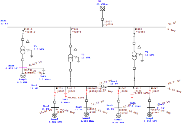
Figure 1. Simulated Single Line Diagram of Borokiri Network Port Harcourt showing the magnitude.

This chapter presents the Earthing System Analysis for Steel Tower Carrying 33kV line, using Borokiri Port Harcourt as a case study. The ETAP and matlab Simulation Results are also presented.

3.1. Parameters Used in the Analysis

Table 12. Simulation parameters used.

Serial No.	Quantity	Value
1	Supply Voltage	415V, 50Hz (line-line)
2	Tower height	18M
3	AC lighting source	10KA
4	Source Impedance	R_s= 0.5 Ω, L_s= 0.1 mH
5	DC Capacitor	5000 uF
6	DC Link Voltage	680V
7	Ripple filter	L_f= 2 mH, C_f= 50 uF
8	Series Transformer	1:1
9	Switching Frequency	20 kHz
10	Load	Three Phase Balanced Linear Load $R - L load (R = 30 Ω, L = 0.302 H)$

Table 13. Showing Resistance, Reactance, and Admittance with Bus Location.

Bus Location	Resistance R (𝛺)	Reactance X (𝛺)	Admittance Y (𝛺)
Okaiki	0.254384	0.150000	0.0000637
Navy Medical	0.254384	0.151000	0.0000637
Navy School	0.254384	0.143000	0.0000660
Wilson Bakery	0.254384	0.127000	0.0000637
Navy Barrack	0.327145	0.150000	0.0000581
Nembe	0.254384	0.143000	0.0000637
Hydro-Graphy	0.254384	0.143000	0.0000637
Egbema	0.637122	0.150000	0.0000498
Immaculate Heart	0.254384	0.143000	0.0000637
Etche Water Front	0.637122	0.150000	0.0000498
Rex Lawson	0.254384	0.143000	0.0000637
Fire Service	0.254384	0.143000	0.0000637
Kolokuma/Etche	0.254384	0.143000	0.0000637
Bori by Anasi	0.254384	0.143000	0.0000637
Oba	0.254384	0.143000	0.0000637
Obina	0.254384	0.143000	0.0000637
Okilopolo	0.254384	0.127000	0.0000660
Inter-lock	0.254384	0.143000	0.0000637
El-Shaddai	0.254384	0.143000	0.0000637
Church of God Mission	0.254384	0.143000	0.0000637
Comprehensive Sec. Sch Gate	0.254384	0.143000	0.0000637
Comprehensive Sec sch. Compound	0.327145	0.151000	0.0000581
New Road By Comp. Sec Sch	0.254384	0.143000	0.0000637
Faith	0.254384	0.143000	0.0000637
Abiye Sekibo	0.254384	0.143000	0.0000637
Greenson I	0.254384	0.143000	0.0000637
Greenson II	0.254384	0.127000	0.0000660
Life Way I	0.254384	0.143000	0.0000637
Life Way II	0.254384	0.143000	0.0000637
Dr. Adoki	0.254384	0.143000	0.0000637
Accountant Estate	0.254384	0.143000	0.0000637
Bob-Manuel	0.254384	0.127000	0.0000660
Jesus Place	0.254384	0.143000	0.0000637
Ikpukulu MTN Mass	0.254384	0.143000	0.0000637

Table 13 shows resistance, reactance and admittance with bus location. From the table, the values of the resistance, reactance and admittance respectively were calculated to determine the voltage drop of each bus location.

3.2. Result Analysis of the Earthing System

Table 14. Earth fault analysis at Borokiri 33kv Bus.

Earthing type	Fault current			Phase voltage
Earthing type	A-phase	B-phase	C-phase	A-phase	B-phase	C-phase
Solidly	3110	0.000	0.000	0.000	7.1045	6.5421
60ohm NEX	850	0.000	0.000	0.000	11.0113	10.1566
30 ohm NER	1750	0.000	0.000	0.000	8.1340	11.4312

The following table shows earth fault current and phase voltages for a simulation of A-phase to ground at Borokiri 33kv Bus with different earthing systems.

Download: Download full-size image

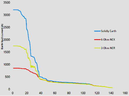
Figure 2. Current value for earthing system analysis for Borokiri.

The Figure 2 above shows the difference in fault current values for A-phase to ground fault simulation on the 33kvv feeder with different earthing system. This was simulated to look at the difference in fault current values.

Download: Download full-size image

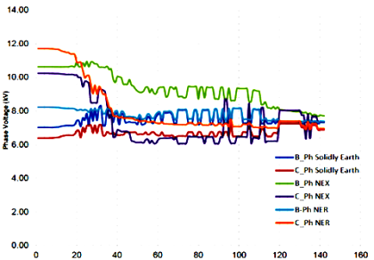
Figure 3. Voltage value for earthing system analysis for Borokiri.

The Figure 3 above shows the difference in Voltage values for A-phase to ground fault simulation on the 33kvv feeder with a different earthing system. The voltages on faulted and unfaulted phases were looked at to understand the effects of earth fault currents on system voltages.

From the above results and analysis, it can be seen that the highest value of fault current (3110A) is obtained from a solidily earthed system. The fault current drops accordingly to the value of resistance or reactance earth system. Phase to phase voltage is high on a resistance or a reactance earth system as seen from the results/analysis above as compared to a solid earth system. The increase in steady state and transient overvoltage caused by impedance earth during an earth fault on the second phase can result in the fault spreading to other phases. The components and hardware used in the systems has to be adequately rated to withstand these transients overvoltage to prevent continuous equipment damages during a fault scenario in other parts of the network.

Download: Download full-size image

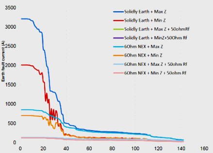
Figure 4. Earth fault current value comparison on 33kv bus feeder.

Download: Download full-size image

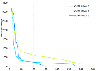
Figure 5. Solidly earth with max source impedance and no fault resistance.

From the fault current it can be seen that for a solidly earthed system and a system with 60 ohm NEX, the fault values are significantly high at source, while the values are significantly small at the remote end or as the fault moves away from the source along the feeder. Since the driving voltage is high and negligible impedance at the source, it contributes to high values of earth fault current at the source. As the fault moves away from the source, the voltage drops and impedance increases along the line, hence the fault current drops. As it can be seen from the figure above, that regardless of the earthing system and fault impedance, the fault values at the very remote end of the feeder are very similar. this is due to the fact that since the fault has moved so far from the source and adding impedance no longer has effect in then fault current. Small values of current at remote ends or along the feeder, if more faults resistance is added which effectively refers to high impedance faults, these values will drop more and will become more challenging for protective devices to defect.

The results of the analysis of various scenarios are represented in graphical format as shown in figures. Figure 5 represents the result analysis for a solidly earth system with maximum source impedance and no fault resistance in the network. Maximum source impedance is obtained whereby the system is operating in a system normal status.

3.3. Supply Voltages

3.3.1. Case I: Balanced Supply Voltage

The voltage across the load is kept constant for different supply voltage disturbances. Once the rated balanced voltage is applied to the load, the injected voltage by the voltage source converter is zero ideally but supplies very small voltage to compensate for the drop in the injection transformer.

The subsequent equations correspond to the balanced source voltage.

v_{sa} = 338.846 \sin (wt)

(20)

v_{sb} = 338.846 \sin (wt)

(21)

v_{sc} = 338.846 \sin (wt)

(22)

Download: Download full-size image

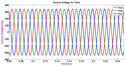
Figure 6. Source Voltage for Balanced Supply Voltage.

Download: Download full-size image

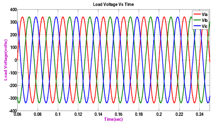
Figure 7. Load Voltage for Balanced Supply Voltage.

Download: Download full-size image

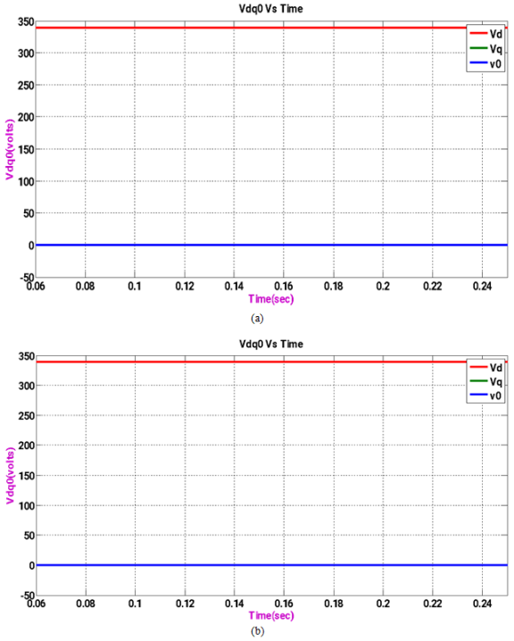
Figure 8. (a), (b) Direct, Quadrature, and Zero axis voltages.

The above figure shows the waveform of Direct, Quadrature, and Zero axis voltages under balanced supply Voltage (simulation is done in Matlab Simulink. The Quadrature and zero axis voltages are of zero voltage after converting the source voltage to a synchronously rotating reference frame (

abc

dq 0

Figure 8a shows the waveform of Balanced Sag Source Voltage (simulation is done in Matlab Simulink). The voltage sag is supplied from 0.08 to 0.2 seconds (6 cycles).

Figure 8b shows the waveform of Load Voltage (simulation is done in Matlab Simulink). The voltage is injected by DVR from 0.08 to 0.2 seconds. From the waveform, it can be observed that the voltage across the load is maintained to rated voltage.

3.3.2. Case II: Balanced Supply Voltage (Sag)

The subsequent equations represent the balanced sag voltage with 20% of sag. The peak value of phase voltage is 338.846V and line to line voltage of 415V.

[16, 17]

v_{sa} = (338.846 * 0.8) \sin \sin (wt)

(23)

v_{sb} = (338.846 * 0.8) \sin \sin (wt - 120)

(24)

v_{sc} = (338.846 * 0.8) \sin \sin (wt - 240)

(25)

Download: Download full-size image

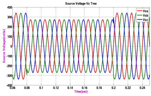
Figure 9. Source Voltage for Balanced Supply Voltage (Sag).

Download: Download full-size image

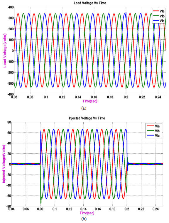
Figure 10. (a), (b) Load voltage for Balanced Supply Voltage (Sag).

Download: Download full-size image

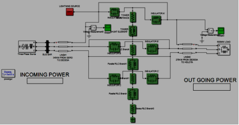
Figure 11. HV Tower model in MATLAB for direct stroke.

Now let's consider the direct stroke case (stroke to phase conductor). In this case the stroke (shown at the top edge of the tower entitled as lightning source) is assumed to strike the phase conductor.

Download: Download full-size image

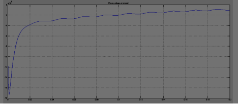
Figure 12. Plot of phase voltage at scope 1 under direct stroke.

From this result it is easy to see that when lightning strikes phase conductor voltage will go far beyond operating voltage for a very short duration of time and then it quickly disappears. In this study lightning source is modeled by using current source of amplitude 20kA in parallel with series RLC branch of 400 ohm to represent surge impedance of the tower. When direct stroke occurred the voltage increased to 17MV and then decayed to about 1MV.

Indirect stroke

This will happen if the lightning strikes shield wire or tower structure.

Download: Download full-size image

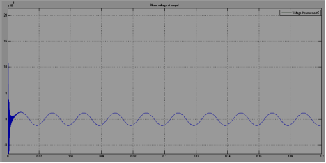
Figure 13. Plot of phase voltage at scope 1 under indirect stroke.

From this it can be concluded that when lightning stroke happens to shield wire or tower body, operating voltage or phase voltage will be decreased as insulator voltage goes beyond operating voltage thereby reducing phase voltage to very small value.

3.4. Transient Simulation of Borikiri Transmission Line

The model described in this section illustrates the protection system of a series compensated transmission system that represents transmission line transmission line which is protected by MOV. The model represents a three-phase, 50 Hz, 500 kV power system transmitting power from a power plant consisting of sixteen 375 MVA generators to an equivalent system through a 220 km transmission line. The transmission line is split into two 245 km and 175 km lines connected between buses B1, B2, and B3. To increase the transmission capacity, each line is series compensated by capacitors representing 50% of the line reactance. The line is also shunt compensated by a 330 MVAr shunt reactance. Each series compensation bank is protected by metal-oxide varistors (MOV). The two circuit breakers of line 1 are shown as CB1 and CB2.

Download: Download full-size image

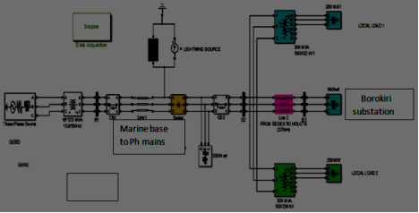
Figure 14. MATLAB model for transient analysis.

Lightning Transient Simulation

Download: Download full-size image

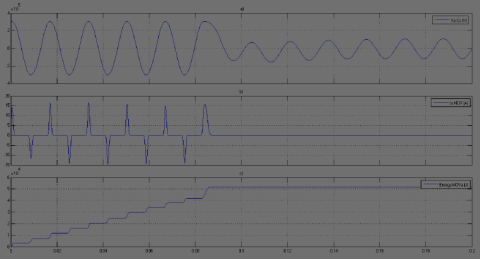
Figure 15. Lightning transient simulation result.

a. Series capacitor voltage,

b. MOV current

c. MOV energy for lightning study

The simulation starts in steady state.

At the t = 1 cycle, lightning stroke is applied and the fault current reaches 10 kA. During the fault, the MOV conducts at every half cycle and the energy dissipated in the MOV builds up to 5MJ.

At t = 5 cycles the line protection relays open breakers CB1 and CB2 and the energy stays constant. At the breaker opening time, the fault current drops to a small value and the line and series capacitance start to discharge through the fault and the shunt reactance. The fault current extinguishes at the first zero crossing after the opening order given to the fault breaker (t = 6 cycles). Then the series capacitor stops discharging and its voltage oscillate.

3.5. Simulation of Transmission Line Protected from Sending and Receiving End by MOV

Below figure shows a 132 kV transmission system with two transmission line arresters placed at the sending end and the receiving end of the line. Over the system a lightning surge of 20 kA was induced and the resulting simulation was carried out by using MATLAB software. A 132 kV transmission system feeds a load (2000MW) through a 220 km transmission line. The result of the simulation shows the temporary increase in current at MOV which is done by the lightning when 20 kA lightning current is applied. On the other hand, the temporary increase in voltage in each arrester.

Download: Download full-size image

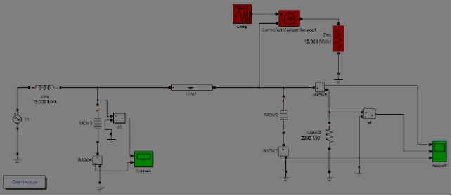
Figure 16. Model to simulate TL protected by MOV.

Here the generation and load are both protected by metal oxide varistors (MOV). The MOV consists of 30 columns protecting the components at 2.5 times its rated voltage. Hence protection voltage is 2.5∗132kV=330kV.

Download: Download full-size image

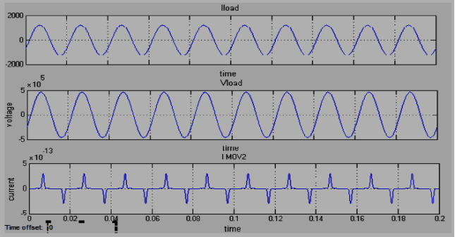
Figure 17. Load current, load voltage, and MOV current under normal conditions.

If stroke happens at receiving end of TL, the resulting current and voltage wave form (without employing MOV Surge arrester) are represented by Figure 17. Initially, the current will raises up to 10kA and the voltage will raises up to 4MV.

Download: Download full-size image

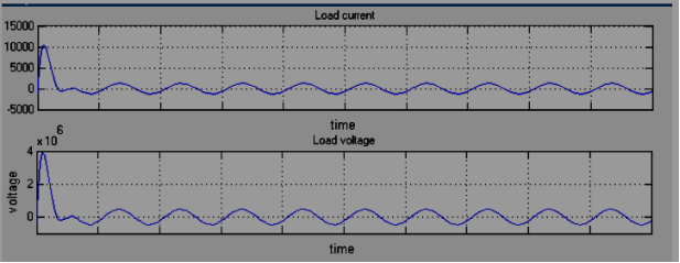
Figure 18. Load current, load voltage, and MOV current when lightning strikes the line If MOV Surge arrester is employed to the system at sending and receiving ends, the current and voltage waveforms look like the following. Initially when the current and voltage wave go to high value, the MOV will conduct until the value drops to tolerable value.

Download: Download full-size image

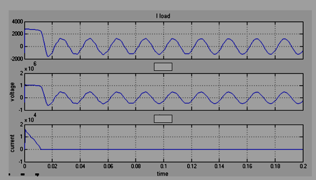
Figure 19. Load current, load voltage, and MOV current after employing Surge arrester.

3.6. Benefits and Challenges of Existing Earthing Systems

Solidly Earth

The main benefits include:

1) Highest magnitude of phase to earth fault currents and simple earth fault protection can be utilised in most places.

2) Overvoltages during earth faults are the lowest (around 0.8 time’s phase to phase voltage).

3) Arcing ground faults cannot occur as the short circuit current is much larger than the capacitive charging and eliminates its influence.

4) Lowest capital and maintenance cost as there is no need for extra equipment to be installed between the transformer neutral terminal and substation earth grid. Simple to understand by operational personnel.

The main challenges include:

1) Presence of high fault currents can cause severe damage to system plants. High fault currents present severe flash and shock hazards.

2) High fault currents can lead to interference in communication circuits in the vicinity of power cables and overhead power lines.

3) Resistance / Reactance Earthing – NER’s & NEX’s The main benefits include: Low magnitude of phase to earth fault currents hence reducing the risk of severe flash hazards. Less likelihood of equipment damage as earth fault current is greatly reduced.

Safer for work personnel and general public in-terms of reduction in step and touch potential.

The main challenges include:

1) High values of transient overvoltages during faults. This needs to be considered carefully in design stages, the rating of surge arresters and short-time thermal current ratings of underground cable screens and earthing conductors.

2) High capital and maintenance cost as equipment needs to be installed between the transformer neutral and substation earth which also needs to be maintained for the life of the equipment.

3) Also high cost of retrofitting on the networks that are not designed to handle the overvoltages.

4. Conclusion

To sum up, our thorough examination of the earthing system for steel towers carrying 33 kV power lines provides important new information about how to improve the dependability and security of power transmission networks. We have offered useful suggestions for enhancing the design of earthing systems by taking into account elements like soil resistivity, tower shape, and grounding electrode combinations. These results are crucial in helping engineers and industry professionals apply robust and efficient earthing systems, which will ultimately improve the lifespan and overall performance of high-voltage power transmission infrastructure. The understanding acquired from this research is crucial for guaranteeing the safe and sustainable operation of 33kV steel tower installations as technology develops and power demands rise.

Conflicts of Interest

The authors declare no conflicts of interest.

References

[1]	Abdulkareem, A. C., Awosope, O. A., Adoghe, A. U. & Alayande, S. A. (2016). Investigating the Effect of Asymmetrical Faults at Some Selected Buses on the Performance of the Nigerian 330-kV Transmission System. International Journal of Applied Engineering Research, 11(7), 5110-5122.
[2]	Abdulkareem, A. C., Awosope, O. A., & Awelewa, A. A. (2016). The use of three-phase fault analysis for rating circuit breakers on Nigeria 330 kV transmission lines. Journal Engineering and Applied Sciences, 11(12), 2612-2622.
[3]	ADENIYI D ADEBAYO and CHINEDU JAMES UJAM (2023) Analysis Of Electrical Grounding Designs Of SubStations And Lines: International Journal Of Scholarly Research In Engineering And Technology, 02(01), 031-040.
[4]	Andrew, A., Sen, P. K. & Clifton, O. (2014). Designing safe and reliable grounding in AC substations with poor soil resistivity: An interpretation of IEEE Std. 80, 1-7.
[5]	Awalin, L., Mokhlis, H. & Abu Bakar, A. H. (2012). Recent Developments in Fault Location Methods for Distribution Networks. Przeglad Elektrotechniczny, 88, 206-212.
[6]	BS 7430 (2011). Code of Practice for Protective Earthing of Electrical Installations.
[7]	Buba, S. D., Wan Ahmad, W. F., Ab Kadir, M. Z. A., Gomes, C., Jasni, J., & Osman, M. (2014). Reduction of Earth Grid Resistance by addition of Earth Rods to various Grid Configurations. ARPN Journal of Engineering and Applied Science. 11(3), 4533-4538.
[8]	Chebbi, S. & Meddeb, A. (2015). Protection plan medium voltage distribution network in Tunisia. International scholarly and scientific Research & Innovation, 9(2), 1307-6892.
[9]	Cifuentes-Chaves, H., Mora-Florez J. & Perez Londoris S. (2017). Time Domain Analysis for Fault Location in Power Distribution System Considering the Load Dynamics. Electrical Power System Research, 146, 331-340.
[10]	Daisy, M. & Dashti, R. (2016). Single Phase Fault Location in Electrical Distribution Feeder Using Hybrid Method. Journal on Energy, 103, 356-368.
[11]	Esobinenwo, C. S., Akinwole, B. O. H., & Omeje C. O. (2014). Earth mat designfor132/33kv substation in Rivers state using ETAP. International Journal of Engineering Trends and Technology (IJETT). 15(8), 389-402.
[12]	Gabrial-Benmou, Y. A. L. (2006). The Protection of Synchronous Generators: In Grigspy, L. L. (Ed.) Electric Power Engineering Handbook-Electric Power Generation, Transmission, and Distribution. CRC press.
[13]	Holtzhausen, J. P. "High Voltage Insulators" (PDF). IDC Technologies. Retrieved 2008-10-17.
[14]	IEC 60137:2003. 'Insulated bushings for alternating voltages above 1,000 V.' IEC, 2003.
[15]	Kakani, L. (2010). Electronics Theory and Applications. New Age International. p. 7. ISBN 978-81-224-1536-0.
[16]	Sarangi, P. P., Sahu, A., & Panda, M. (2013). A Hybrid Differential Evolution and Back Propagation Algorithm for Feedforward Neural Network Training. International Journal of Computer Applications, 84, 1-9. http://doi.org/10.5120/14641-2943
[17]	Usman I. A, (2015). A design of protection schemes for AC Transmission lines considering a case study. International Journal of Electrical and Electronics Engineers, 7(2).

Cite This Article

Plain Text BibTeX RIS

APA Style

David, A. A., Ncheta, I. E., Rufus, O. O. (2024). Earthing System Analysis for Steel Tower Carrying 33kV Line. Engineering Science, 9(2), 21-38. https://doi.org/10.11648/j.es.20240902.11

Copy | Download

ACS Style

David, A. A.; Ncheta, I. E.; Rufus, O. O. Earthing System Analysis for Steel Tower Carrying 33kV Line. Eng. Sci. 2024, 9(2), 21-38. doi: 10.11648/j.es.20240902.11

Copy | Download

AMA Style

David AA, Ncheta IE, Rufus OO. Earthing System Analysis for Steel Tower Carrying 33kV Line. Eng Sci. 2024;9(2):21-38. doi: 10.11648/j.es.20240902.11

Copy | Download

@article{10.11648/j.es.20240902.11,
  author = {Adebayo Adeniyi David and Ifeagwu Emmanuel Ncheta and Ogunsakin Olatunji Rufus},
  title = {Earthing System Analysis for Steel Tower Carrying 33kV Line
},
  journal = {Engineering Science},
  volume = {9},
  number = {2},
  pages = {21-38},
  doi = {10.11648/j.es.20240902.11},
  url = {https://doi.org/10.11648/j.es.20240902.11},
  eprint = {https://article.sciencepublishinggroup.com/pdf/10.11648.j.es.20240902.11},
  abstract = {This study examines the critical analysis of earthing systems connected to steel towers that carry 33 kV power lines. Ensuring the safety and dependability of power transmission infrastructure becomes crucial in light of the growing demand for energy. By utilizing sophisticated computational methodologies and simulation approaches, this research carefully investigates how well the earthing system performs in various operational circumstances and fault scenarios. A thorough modeling technique is used in the analysis, which considers a number of variables including fault currents, tower design, soil resistivity, and grounding electrode configurations. In order to give a comprehensive understanding of the behavior of the system and its consequences for operational reliability, the study simulates many situations, including normal operation and fault occurrences. By using sophisticated numerical simulations and sensitivity analysis, the research pinpoints important factors affecting the earthing system's efficiency and suggests creative optimization techniques. These optimization techniques could involve changing the location of the grounding electrode, improving the materials used in the conductor, or putting additional safety precautions in place. The researcher's conclusions have important ramifications for the engineering community since they provide practical advice on how to strengthen the security and robustness of power transmission networks. The study adds to the continuous efforts to improve the efficiency and dependability of electrical grids by addressing potential weaknesses in the architecture of the earthing system. This thorough study advances the field of earthing system engineering by offering a solid platform for next studies and real-world implementations. Through this work, we can better understand the dynamics of earthing systems and optimization methodologies, which will help build more resilient and sustainable power transmission infrastructure that can adapt to society's changing energy needs.
},
 year = {2024}
}

Copy | Download

TY  - JOUR
T1  - Earthing System Analysis for Steel Tower Carrying 33kV Line

AU  - Adebayo Adeniyi David
AU  - Ifeagwu Emmanuel Ncheta
AU  - Ogunsakin Olatunji Rufus
Y1  - 2024/06/29
PY  - 2024
N1  - https://doi.org/10.11648/j.es.20240902.11
DO  - 10.11648/j.es.20240902.11
T2  - Engineering Science
JF  - Engineering Science
JO  - Engineering Science
SP  - 21
EP  - 38
PB  - Science Publishing Group
SN  - 2578-9279
UR  - https://doi.org/10.11648/j.es.20240902.11
AB  - This study examines the critical analysis of earthing systems connected to steel towers that carry 33 kV power lines. Ensuring the safety and dependability of power transmission infrastructure becomes crucial in light of the growing demand for energy. By utilizing sophisticated computational methodologies and simulation approaches, this research carefully investigates how well the earthing system performs in various operational circumstances and fault scenarios. A thorough modeling technique is used in the analysis, which considers a number of variables including fault currents, tower design, soil resistivity, and grounding electrode configurations. In order to give a comprehensive understanding of the behavior of the system and its consequences for operational reliability, the study simulates many situations, including normal operation and fault occurrences. By using sophisticated numerical simulations and sensitivity analysis, the research pinpoints important factors affecting the earthing system's efficiency and suggests creative optimization techniques. These optimization techniques could involve changing the location of the grounding electrode, improving the materials used in the conductor, or putting additional safety precautions in place. The researcher's conclusions have important ramifications for the engineering community since they provide practical advice on how to strengthen the security and robustness of power transmission networks. The study adds to the continuous efforts to improve the efficiency and dependability of electrical grids by addressing potential weaknesses in the architecture of the earthing system. This thorough study advances the field of earthing system engineering by offering a solid platform for next studies and real-world implementations. Through this work, we can better understand the dynamics of earthing systems and optimization methodologies, which will help build more resilient and sustainable power transmission infrastructure that can adapt to society's changing energy needs.

VL  - 9
IS  - 2
ER  -

Copy | Download

Author Information

Adebayo Adeniyi David

Department of Electrical and Electronic Engineering, Federal University, Otuoke, Nigeria

Contact Email

http://orcid.org/0000-0002-9959-9927
Ifeagwu Emmanuel Ncheta

Department of Electrical and Electronic Engineering, Federal University, Otuoke, Nigeria

Contact Email
Ogunsakin Olatunji Rufus

Department of Information and communication (I.C.T), Federal University, Otuoke, Nigeria

Contact Email

Download PDF

Submit an Article

Plain Text BibTeX RIS

APA Style

David, A. A., Ncheta, I. E., Rufus, O. O. (2024). Earthing System Analysis for Steel Tower Carrying 33kV Line. Engineering Science, 9(2), 21-38. https://doi.org/10.11648/j.es.20240902.11

Copy | Download

ACS Style

David, A. A.; Ncheta, I. E.; Rufus, O. O. Earthing System Analysis for Steel Tower Carrying 33kV Line. Eng. Sci. 2024, 9(2), 21-38. doi: 10.11648/j.es.20240902.11

Copy | Download

AMA Style

David AA, Ncheta IE, Rufus OO. Earthing System Analysis for Steel Tower Carrying 33kV Line. Eng Sci. 2024;9(2):21-38. doi: 10.11648/j.es.20240902.11

Copy | Download

@article{10.11648/j.es.20240902.11,
  author = {Adebayo Adeniyi David and Ifeagwu Emmanuel Ncheta and Ogunsakin Olatunji Rufus},
  title = {Earthing System Analysis for Steel Tower Carrying 33kV Line
},
  journal = {Engineering Science},
  volume = {9},
  number = {2},
  pages = {21-38},
  doi = {10.11648/j.es.20240902.11},
  url = {https://doi.org/10.11648/j.es.20240902.11},
  eprint = {https://article.sciencepublishinggroup.com/pdf/10.11648.j.es.20240902.11},
  abstract = {This study examines the critical analysis of earthing systems connected to steel towers that carry 33 kV power lines. Ensuring the safety and dependability of power transmission infrastructure becomes crucial in light of the growing demand for energy. By utilizing sophisticated computational methodologies and simulation approaches, this research carefully investigates how well the earthing system performs in various operational circumstances and fault scenarios. A thorough modeling technique is used in the analysis, which considers a number of variables including fault currents, tower design, soil resistivity, and grounding electrode configurations. In order to give a comprehensive understanding of the behavior of the system and its consequences for operational reliability, the study simulates many situations, including normal operation and fault occurrences. By using sophisticated numerical simulations and sensitivity analysis, the research pinpoints important factors affecting the earthing system's efficiency and suggests creative optimization techniques. These optimization techniques could involve changing the location of the grounding electrode, improving the materials used in the conductor, or putting additional safety precautions in place. The researcher's conclusions have important ramifications for the engineering community since they provide practical advice on how to strengthen the security and robustness of power transmission networks. The study adds to the continuous efforts to improve the efficiency and dependability of electrical grids by addressing potential weaknesses in the architecture of the earthing system. This thorough study advances the field of earthing system engineering by offering a solid platform for next studies and real-world implementations. Through this work, we can better understand the dynamics of earthing systems and optimization methodologies, which will help build more resilient and sustainable power transmission infrastructure that can adapt to society's changing energy needs.
},
 year = {2024}
}

Copy | Download

TY  - JOUR
T1  - Earthing System Analysis for Steel Tower Carrying 33kV Line

AU  - Adebayo Adeniyi David
AU  - Ifeagwu Emmanuel Ncheta
AU  - Ogunsakin Olatunji Rufus
Y1  - 2024/06/29
PY  - 2024
N1  - https://doi.org/10.11648/j.es.20240902.11
DO  - 10.11648/j.es.20240902.11
T2  - Engineering Science
JF  - Engineering Science
JO  - Engineering Science
SP  - 21
EP  - 38
PB  - Science Publishing Group
SN  - 2578-9279
UR  - https://doi.org/10.11648/j.es.20240902.11
AB  - This study examines the critical analysis of earthing systems connected to steel towers that carry 33 kV power lines. Ensuring the safety and dependability of power transmission infrastructure becomes crucial in light of the growing demand for energy. By utilizing sophisticated computational methodologies and simulation approaches, this research carefully investigates how well the earthing system performs in various operational circumstances and fault scenarios. A thorough modeling technique is used in the analysis, which considers a number of variables including fault currents, tower design, soil resistivity, and grounding electrode configurations. In order to give a comprehensive understanding of the behavior of the system and its consequences for operational reliability, the study simulates many situations, including normal operation and fault occurrences. By using sophisticated numerical simulations and sensitivity analysis, the research pinpoints important factors affecting the earthing system's efficiency and suggests creative optimization techniques. These optimization techniques could involve changing the location of the grounding electrode, improving the materials used in the conductor, or putting additional safety precautions in place. The researcher's conclusions have important ramifications for the engineering community since they provide practical advice on how to strengthen the security and robustness of power transmission networks. The study adds to the continuous efforts to improve the efficiency and dependability of electrical grids by addressing potential weaknesses in the architecture of the earthing system. This thorough study advances the field of earthing system engineering by offering a solid platform for next studies and real-world implementations. Through this work, we can better understand the dynamics of earthing systems and optimization methodologies, which will help build more resilient and sustainable power transmission infrastructure that can adapt to society's changing energy needs.

VL  - 9
IS  - 2
ER  -

Copy | Download